A hash function is a map from a domain $[n]$ to a codomain $[m]$, written as $h: [n]\to [m]$. We want the output to look random. For a fixed function $h$ and a fixed input $x$, the output $h(x)$ is fixed. We therefore introduce randomness by choosing $h$ from a family of hash functions $\mathcal{H}$.
There are $m^n$ functions from $[n]$ to $[m]$, so representing an arbitrary such function requires $\Omega(n\log_2m)$ bits. In many applications, it suffices that, for any $k$ distinct inputs $x_1,x_2,\ldots,x_k\in [n]$, the outputs $h(x_1),h(x_2),\ldots,h(x_k)$ are independent and uniformly distributed over $[m]$, where $h$ is chosen uniformly from $\mathcal{H}$. Such a family is called $k$-wise independent. Equivalently, assuming $1\leq k\leq n$, we have
\[\Pr_{h\sim\mathcal H} [h(x_1)=y_1,\ldots,h(x_k)=y_k]=m^{-k},\]for every choice of distinct inputs and every output tuple.
Such a family can be constructed using polynomials over a finite field $F\cong \mathbb{F}_q$ of size $q=m=n$. Specifically, we take
\[\mathcal{H}:=\lbrace f\in F[X]_{<k}\rbrace.\]Here I’d like to highlight the elegant algebraic structure.
Randomness
Fixing any $\alpha\in F$ gives us an evaluation map
\[\begin{align*} &\phi_\alpha: \mathcal{H}\to F,\\ &\phi_\alpha: f\mapsto f(\alpha). \end{align*}\]This is a homomorphism under addition (more precisely, it is a linear transformation). It is surjective because, for any $\beta\in F$, the constant polynomial $f(X)=\beta$ satisfies $f(\alpha)=\beta$. Its kernel is a subspace of $\mathcal{H}$, and each fibre is a coset of this kernel. All $q$ fibres therefore have the same size, so $f(\alpha)$ is uniformly distributed over $F$ when $f$ is chosen uniformly from $\mathcal{H}$.
Independence
One way to establish independence is to use the full-rank property of the Vandermonde matrix; we leave this as an exercise for the reader.
Fix distinct evaluation points $\alpha_1,\ldots,\alpha_k\in F$. Let us first ask for all the evaluations to be zero. Starting with $H_0=\mathcal{H}$, each new condition selects the kernel of the next evaluation map: $H_i=\ker(\phi_{\alpha_i}\mid_{H_{i-1}})$. We obtain a chain of subspaces:
\[\mathcal{H}=H_0\supseteq H_1\supseteq\cdots\supseteq H_k.\]At each step, the restricted evaluation map is still surjective1. By the argument from the previous section, it partitions $H_{i-1}$ into $q$ equally sized cosets of $H_i$. Choosing the value zero selects the kernel itself. We are back in a subspace, so the same picture repeats inside it.
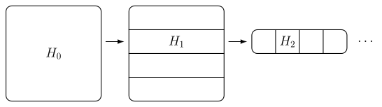
What changes if the prescribed values $\beta_i$ are not all zero? The remaining polynomials now form a translate $f_{i-1}+H_{i-1}$, an affine subspace. Evaluation on this translate simply adds the fixed offset $f_{i-1}(\alpha_i)$ to the linear map on $H_{i-1}$. The fibres are still cosets of $H_i$, all of the same size; fixing the next value selects one of them, giving $f_i+H_i$. The recursive structure is unchanged.
Thus, whether we select the kernel or one of its translates, each successive condition retains a fraction $1/q$ of the remaining polynomials. For any $\beta_1,\ldots,\beta_k\in F$, this gives
\[\Pr_{f\sim\mathcal H} [f(\alpha_1)=\beta_1,\ldots,f(\alpha_k)=\beta_k] =q^{-k}.\]-
The polynomial $\prod_{j<i}(X-\alpha_j)$ has degree $i-1<k$, belongs to $H_{i-1}$, and is nonzero at $\alpha_i$. Its scalar multiples therefore attain every value in $F$ at $\alpha_i$. For $i=1$, the empty product is $1$. ↩
·